It's Common to Overstate Measurement Precision

It's often the case that we have a false or unrealistic impression of our measurement capability or the capability of the instruments that we use. Naively, we tend to look at the smallest unit a measurement system can detect and assume that it represents its overall measurement error.

Luckily, there are some simple techniques to test the accuracy of your measurements, and these are well worth learning. This article will show you how to apply some simple analysis techniques to validate your real measurement capability.

In the first part, we'll see a simple analysis of an automated measurement process, and then a more advanced analysis with human operators.

Measurement Systems Analysis (MSA) will provide a capability analysis of any measurement system. There are two major benchmarks to consider: First, that measurement precision is capable of maintaining process control. Second, that measurement precision is capable of maintaining product quality.

Part 1. Studying an Automated Measurement Process

A simple study of this kind would consider one component and measure it 30 times. The standard deviation from a sample of 30 measurements gives you a quick and reliable understanding of your instrument's repeatability between measurements.

The definition of repeatability is simply the error in repeated measurements with a single instrument and a single operator.

An Example Study (without Operator Interaction)

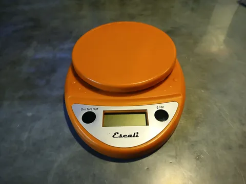
I'll use an inexpensive digital kitchen scale to weigh 1kg of apples. This will serve as an example to show you how to collect the data and analyse it for repeatability. In this case, there is no operator interaction or influence on the measurement; it is fully automated.

The 30 measurements I collected had a standard deviation of 0.714g. To calculate this yourself, use Microsoft Excel, Google Sheets, or the equivalent, using the built-in formula STDEV.S([range]).

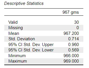
With the assumption that this measurement process is normally distributed, an estimate of the range of measurement error can be calculated from six times the measurement standard deviation (where six standard deviations will cover 99.7% of all measurements). Calculating 6 × 0.714g yields 4.284g, which is more than four times the 1g resolution of our scales, much more than we may have naively assumed.

I've provided the raw data so you can test this yourself. This should also allow you to collect and substitute your own data.

Download CSV

Establishing the Measurement Protocol

We should establish a measurement protocol that is consistent. For kitchen scales, measurements are normally started from the powered-down state. An example measurement protocol could then be:

1. Switch the scales on
2. Zero or tare the scales
3. Load the scales in the same way with the item, or items
4. Wait for the reading to stabilise
5. Turn off the scales after taking the measurement

You should go through this full cycle each time to be representative of a single measurement.

Measurement Capability vs. Product Quality

Assume we are packing 1kg of apples where the process variation is 50g and the production tolerance is 100g. (This is the ideal case where process variation is twice as good as the customer specification) The standard benchmarks are any measurement error should be less than 10% of the process variation and less than 10% of the production tolerance.

Our measurement system repeatability error was 4.284

4.284 ÷ 50 = 8.6% of the process variation

4.284 ÷ 100 = 4.3% of the tolerance

Both of these benchmarks suggest an adequate measurement system

However, if we were to use the same scale to pack another product, where the process variation is 5g and the tolerance is only 10g, then our repeatability error would be entirely unacceptable

The target of 10% for these benchmarks can be relaxed, but only for processes that are highly capable and under good control. In that case there would be a very low probability of an out of specification product and therefore the need for precision in preventing the escape of defects to customers is less critical.

Measuring and improving process capability is not a topic we will cover now, but it would be well covered by any Lean Six Sigma Green Belt course.

Part 2. Studying a Manual Measurement Process

This training example uses ten coins measured in random order, then repeated in a different random order. That provides ten pairs of measurements to assess the repeatability of measurement. If we also have two or more operators run the same trial, we can calculate the reproducability between operators.

Repeatability & Reproducibility

The definition of repeatability is simply the error in repeated measurements with a single instrument and a single operator.

Reproducibility in MSA is used to describe the error in measurement that is introduced by using different operator

Blind trial

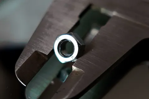
If I were to ask you to measure the diameter of a coin using a vernier calliper, you could probably do that with a little practice.

If I ask you to do that 30 times, you will likely give me 30 identical measurements. You know the correct answer from your first measurement, so your following measurements will be influenced by that knowledge.

To remove that bias, we need to structure the trial to eliminate that prior knowledge. Whenever there is human operator interaction with the instrument, we will need a randomised blind trial.

Measurement Protocol

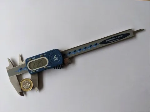
We'll use a digital calliper to measure the width of a random sample of ten coins of the same kind. To preserve the blind trial, we need to apply a serial number to each coin. Each coin can be placed on a table with a unique serial number from 1 to 10, on the hidden face.

The data collector arranges the coins in a random order that only he or she knows, and each operator measures them independently without conferring, giving the measurement to the data collector. They shuffle the coins and each operator measures them a second time, with the data again collected by the data collector.

Ideally, use flat-edged rather than milled coins. Preserve the orientation to measure the same feature to avoid any ovality contributing to the measurement error. One way to do that is to keep the coin in the same orientation.

Apply a standard light pressure to the calliper using the thumb wheel and grip the coin in the flat part of the jaws without tilting the coin.

Data Collection

We now have ten independent sets of two measures for each serial number. We usually repeat this process for a total of three independent operators. This allows us to calculate both the repeatability and the reproducibility errors in our measurement system using a technique called analysis of variance (ANOVA).

For this, we need to use a statistics package, such as the open-source JASP.

A typical operator measurement study would involve ten components selected at random, with three operators and two repeats of each measurement. This gives us 60 data points and provides sufficient data for a successful ANOVA.

The sample of 60 should be regarded as a minimum. If you only have two operators, then use 15 or 20 parts to keep the data set large.

In this example, I'll use British one-pence coins, which are cheap, accurate and readily available. I can get a hundred very precise components for only £1.

Data Analysis

Let's assume that the manufacturing specification for the diameter of a one-pence coin is 20.3 – 20.4, a tolerance of 0.1mm. Compare this to the resolution of a digital calliper at 0.01mm. This 10-to-1 factor suggests this would be a suitable instrument to control and inspect pennies.

To test this naïve assumption I conducted an MSA study using a sample of 10 pennies measured by three operators with a digital caliper. The data was collected in a CSV file, which will accompany this article.

Download CSV

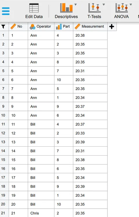
I'll use JASP to analyse the data. You can install the software and then open the CSV file yourself. You should see the measurement data appear in the JASP data tab.

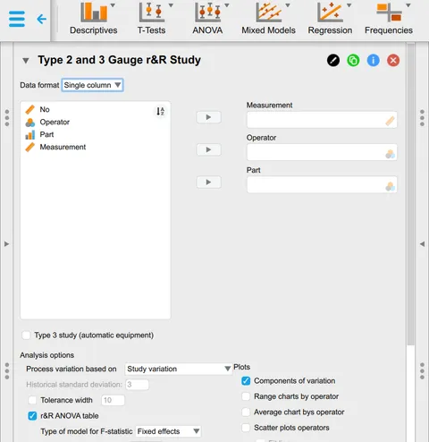
This analysis requires the Quality Control JASP module. You may need to load that first using the blue plus sign on the menu toolbar. Under "Quality Control", select "Measurement Systems Analysis" and then "Gauge r&R Study".

Note that JASP recognises the data types and labels them with a ruler for a continuous variable, a bar chart for an ordinal variable, and three circles for an attribute variable. There are 60 rows of data in total, with operators Alice, Barry, and Colin measuring twice each of the ten parts. The order is randomised, but the software will accept any order and sort the data internally.

In the Gauge r&R analysis dialogue, identify the data fields of interest by dragging them into the three fields for "Measurement", "Operator" and "Part". This directs JASP to extract and process the data for analysis.

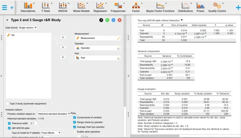
Select additional analysis options: Set the historical standard deviation to 0.038 - this implies that we have long-term data for the process variation. This is a much better benchmark than simply using the standard deviation calculated from a sample of 10. Set the tolerance width of 0.1 for another benchmark and is based on the specification 20.3 -20.4. The various plot options provide clear visual representations of the measurement error compared to those benchmarks, as well as identifying spikes or unusual data that might need to be re-measured.

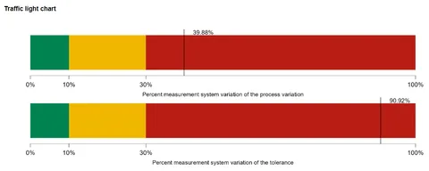
A review of the traffic light chart gives a quick overview of the measurement capability compared to the benchmarks. Both are in the unacceptable region at 35% and 80%. Ideally, they should both be in the under 10% range.

Review of the gauge evaluation data table confirms these results but the numerical data is more difficult to assess that the graphical results.

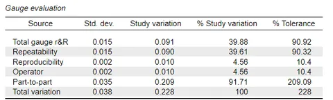
The total gauge r&R represents the combination of both repeatability and reproducibility. It shows as 40% of the Process Variation (called Study in JASP) and 90% of the Tolerance. The same data indicated in the Traffic Light Chart. Bearing in mind the target of 10 % this is clearly an inadequate measurement system.

It also shows that repeatability is the greatest source of error. The reproducibility component is very small. There are little or no discernible differences between operators, most of the error is due to the repeatability of the instrument. An obvious conclusion is that training for operators will have little or no improvement effect, and that buying a better instrument is likely to be the only way to improve measurement capability.

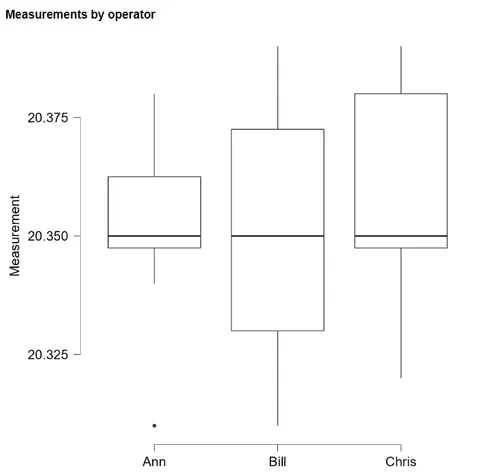
The box and whisker plot compares the measurements of the three operators. With the relatively small samples caution should be used in interpreting these as showing significant differences.

This is a relatively simple analysis to do with the aid of free, open-source software. The data collection needs to be completed with care and is a little time-consuming. Actual data collection in this training example took around 20 minutes. It does provide a useful and realistic appraisal of your true measurement capability and can dispel previously held assumptions and, in some cases, misplaced confidence. It is well worth your time in developing confidence with this MSA technique to be able to train your operators in using it.